A Bestiary of Functions for Systems Designers
Whether your game surfaces its numbers to the player or not, odds are it has underlying systems that rely on them, and you use functions to determine how those numbers affect each other. In other words, a mathematical function is usually at the core of the answer to a bunch of frequent game design questions.
- If I increase my strength, how much does my damage grow?
- How fast does damage fall off when shooting a gun outside its normal range?
- How much more expensive is each subsequent upgrade?
- How aggressively does the AI respond to this stimulus?
- How much XP to the next level?
- How fast does the difficulty ramp up in Infinite Mode?
- How much harder do enemies hit in each New Game+?
- How does the player character’s speed change when the sprint button is held?
- How do quest rewards ramp up over the course of the game?
- How much time do I expect players to spend on each level?
And so on. Sometimes those questions are about the explicit math undergirding game rules; sometimes they’re more about analysis and intent, about the spreadsheet you’re building to later turn into a loot or progression table that the game will express in some other way.
This isn’t meant as a comprehensive primer on those functions let alone some sort of taxonomy. It’s more a collection of interesting specimens, alongside histories, use cases, and observations on their behavior.
A note about mathematics
There are some mentions here of calculus and some potentially scary notation like \(\frac{d}{dx}\), but hopefully the main gist of everything should be understandable as long as you’re familiar with the idea of functions and the most common mathematical notation. If any part of this is very unclear or you think I’ve made a math error (which is very likely!), a good place to ask me questions is actually on tumblr.
Conventions in this article
The word parameter has different meaning to programmers and mathematicians. Usually, in programming, we think of any input of a function as a parameter; if I define a function like (x) -> pow(x, a), we think of x as the parameter and a as some constant defined elsewhere in the code.
In mathematics it’s basically the other way around. Parameters are known or constant values for a given “version” of a function, and the inputs of the function are arguments. So in math, if I define a function like \(f(x) = x^a\), then a is the parameter.
So instead of talking about parameters, I’ll be talking about arguments (the variables that go into a function) and coefficients (the constant values that adjust a function) instead.
For variables, I’ll follow the usual mathematical convention that arguments are usually \(x, y,\) or \(z\). Anything else is a coefficient; \(a, b, c\) are usually additive or multiplicative, \(s\) is usually an exponent, \(k\) is usually a counting number.
The Functions
The Linear Function
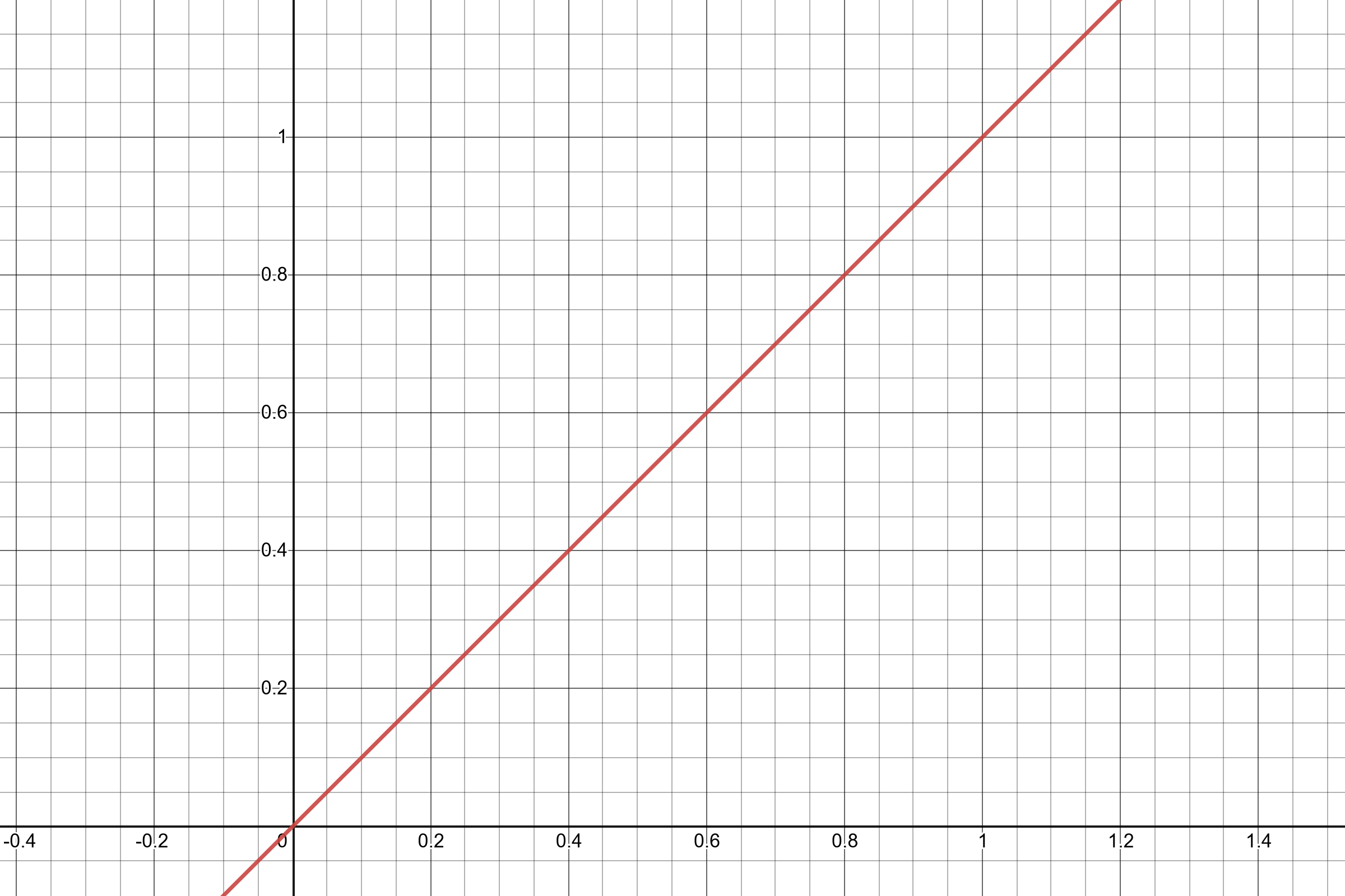
Let’s first establish a baseline by talking about the simplest function, \(f(x) = bx + a\). This is useful to point out the basics of parametrization – by adjusting \(b\), we can change the function’s slope to make it steeper or shallower; by adjusting \(a\) we can shift the output up or down by some amount.
The main reason to use a linear curve is simplicity and clarity. Players can grasp a linear system pretty intuitively, and those functions will hold to several properties that players will expect. For example, if you double \(x\), then \(f(x)\) will also double. If you increase \(x\) by some value \(y\), then \(f(x)\) will increase by the same amount no matter what \(x\) was. This kind of clarity can be invaluable to players who are trying to optimize something.
This simplicity, of course, precludes more complex behaviors. In a lot of game systems, players won’t be cognizant of the underlying numbers and will be learning how the system works by “feel” – in which case, using an easily graspable linear function might not even be any more clear to the player at all. And of course sometimes we don’t want game systems to be immediately clear.
For the rest of these functions, I’ll usually be skipping over various multiplicative and additive coefficients you can throw into these functions to shift or scale their outputs, just so we don’t get lost in symbolic soup.
Quadratic, Cubic, and other Power Functions
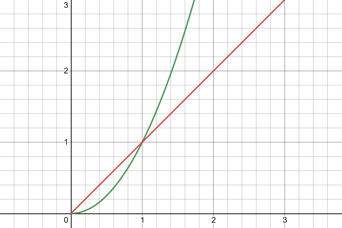
There are several “families” of power functions but at first we should talk about \(f(x) = x^b\), where \(b\) is some small counting number greater than 1, like 2, 3, or 4.
Power functions “feel” very different in the range \(0 \leq x \leq 1 \) than they do when \(x \gt 1\). Inside the unit square, they “bulge” down and away from the linear function, meeting at the 0 and 1 points. Outside that square, \(f_{\mathrm{linear}}(x) \lt f_{\mathrm{quadratic}}(x)\), and the slope increases to infinity.
If you expect a normalized input where \(0 \leq x \leq 1\), power functions are often used to add “juice” to animations or character movement, as easing functions, and so on.
The “outer” range where \(x \gt 1\) is more interesting in designing systems. Power functions give you accelerating growth, which feels powerful for players and, indeed, is inherently dangerous.
Say the player character’s damage and enemy hit points both scale exponentially with their level; say \(f_\mathrm{damage}(x_\mathrm{level}) = x_\mathrm{level}^2\). In practice, the game stays at the same balance if the player is of the same level as the enemies, but the numbers grow explosively. As we know, player happy when number big; this is the kind of thing that works well for games with visible damage numbers.
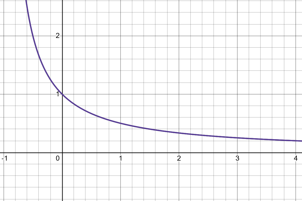
However, as the player gains levels, each subsequent level is a little less significant. You can understand why by looking at a graph of \(\frac{f(x)}{f(x) + 1}\):
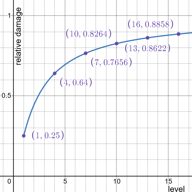
A level 1 player fighting a level 2 enemy might as well be doing 25% damage, whereas the difference between level 10 and level 11 is nowhere near as dramatic. This isn’t nearly as noticeable if x is always a bigger integer, of course, but it’s still there.
In calculus terms, \(\ddx f(x)\) increases as \(x\) increases, but not as fast as \(f(x)\) increases. So while each subsequent level has a bigger absolute effect, in relative terms the percent increase in damage from one level to the next is slowing down.
Everything is relative, so the “feel” of a growth curve will depend on what it’s being compared against. To illustrate this with power curves, consider an RPG where:
- As the player increases in level and enters higher-level content, quest rewards (in money) scale quadratically;
- The prices of consumables stay constant;
- The prices of equipment grows linearly;
- The cost of resurrecting a dead party member grows quadratically;
- The cost of retraining your character grows cubically.
You can see how all those things interact:
- Consumables quickly become unlimited, at least as far as money is concerned. After a few levels you can buy as many potions as you need.
- Equipment becomes cheaper relative to quest rewards, though higher-level equipment is still meaningfully more expensive than low-level equipment. If overleveled equipment is available to buy, it becomes more and more affordable.
- If you lose a party member, the level of effort to pay for their resurrection is always about the same.
- Retraining your character becomes ever more onerous as the game goes on.
These kinds of relationships, of course, emerge from using any function against any other function. It’s very useful to look at the ratios between different functions at different stages of the game, and using those relationships is very important in achieving whatever player experience goals you have.
Fractional and negative powers
Reconsidering \(f(x) = x^s\), we obviously can look at exponents other than 2, 3, and 4. It’s very common to use a value of \(s\) that’s a fractional number to fine-tune the curve and make it exactly as dramatic as intended.
But there are two other useful cases. The first is when \(s\) is some fractional number between 0 and 1. These are diminishing returns functions, where the rate of change decreases as \(x\) increases, but \(f(x)\) keeps increasing forever.
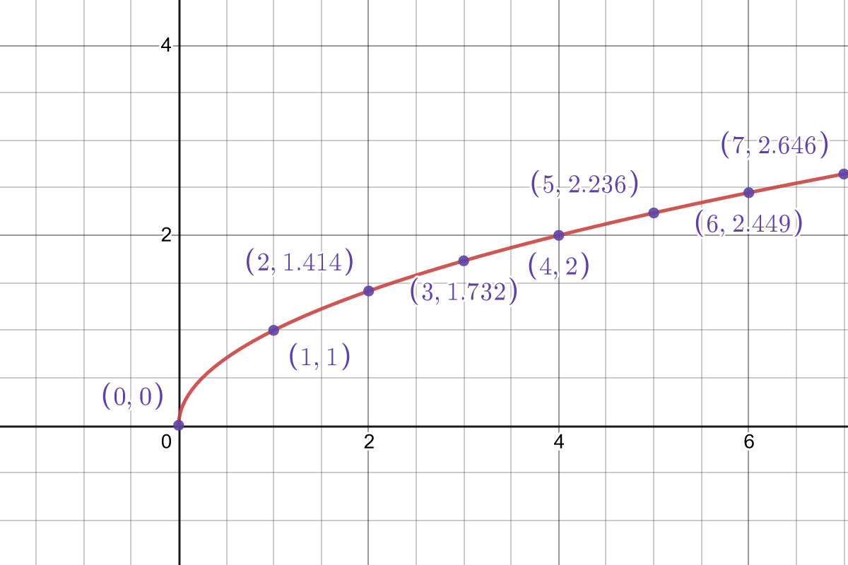
This kind of function has many, many applications. First of all, it front-loads the effect of \(x\); you get the most benefit from having a little of it, instead of stacking a lot of it. A good use for this might be something like damage reduction. Say you can equip a certain amount \(x\) of cold-resistant items, and all together they negate \(10x^{0.5}\) cold damage. Your first cold-resistant item negates 10 damage. But to double that protection and negate 20 damage, you have to quadruple the number of cold-resistant items you have equipped. Putting on another warm pair of mittens, thermal vest, or ushanka will always increase the amount of damage reduction the player gets, but having some is vastly more important and noticeable than having a lot.
Finally, we come to negative powers. If you don’t remember how negative powers work: raising something to a negative power is the same thing as taking the inverse of a positive power; that is:
\[x^{-s} = \frac{1}{x^s}\]
The latter might be easier to reason about, and is probably computationally faster, if that matters for your application.
Note that for a function like \(f(x) = x^{-s}\), the value for \(x = 0\) is undefined, and it approaches infinity. This tends to not be useful, so you will usually see this in the form \(f(x) = (x + 1)^{-s}\), which normalizes it so that \(f(0) = 1\).
You can think of this as an easing-out function; it slows down as \(x\) increases, though it never quite plateaus. Effects are very front-loaded; in the graph above, the first point of \(x\) will halve \(y\), but subsequent points are nowhere near as efficient. But the time we’re at 4, effects are pretty marginal.
The clearest use case for this is as a multiplier for something else which reduces it – giving the player a discount based on their Barter skill, reducing incoming damage based on their armor, and so on. Because of its slowing-down nature, it’s useful for negative effects that can be stacked – for example, reducing the player’s speed as they accumulate stacks of a debuff. Subsequent stacks will always have an effect, but the majority of the impact comes from the first one.
For this article, I’m not really thinking about performance considerations, but they might matter in your game; if a function has to run hundreds of times a second, that might constrain what operations you can really use, depending on context.
As a rule, addition, subtraction, and multiplication are safe to use; division and raising things to fractional or negative powers are computationally expensive.
Exponential Growth
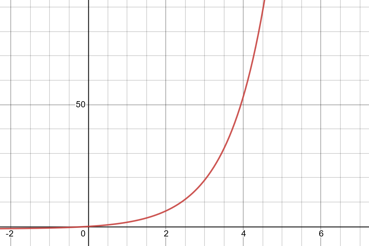
The exponential function, \(f(x) = b^x\), in which \(b \gt 1\). Shown above, specifically, is \(e^x - 1\).
Like the power functions, the exponential function grows to infinity. Unlike with the power function, the rate of growth keeps accelerating in pace with the growth of the value itself, so the relative multiplicative value of each increase stays the same.
Or, again in calculus terms, \(\ddx f(x)\) is just some multiple of of \(f(x)\), such that \(\frac{\ddx f(x)}{f(x)}\) stays constant.
Exponential growth blows up even more than quadratic or cubic growth; if those functions created big, player-pleasing numbers, exponential functions are liable to create even bigger ones. It may make sense to use an exponential function when:
- You want the numbers to truly explode. Maybe you’re exposing them to the player and your game is about seeing that giant pile of zeroes. Maybe your game deals with a huge range of scales. Maybe the input has a small range but you want that small range to translate into dramatic changes in output.
- Example: An idle game like Cookie Clicker, where the numbers exploding is the point.
- Example: A comical physics-driven golf game where the joke is that the 9-iron shoots the ball \(2^9\) times further than the 0-iron.
- You want multiplicative consistency; that is, the absolute increase when you increase the input will grow, but the ratio between level 10 and level 11 is the same as the ratio between level 1 and level 2.
- You’re not worried about game balance, either because the input of the function is strictly bounded, or because you just don’t care.
- Example: Player hit point growth is exponential, but the base is small and the game has a level cap, so we know what the min and max values are.
- Example: Again, an idle game where the joke is that the numbers explode and are unbounded, until the game itself breaks.
Keep in mind that while exponential curves usually look like very sharp “hockey stick” curves, you can have a shallow exponential curve! Just use a base that’s barely above 1. Say you use exponential scaling for the player’s hit points, based on their level, and your game is capped at 20 levels. You can define a function like \(f(x) = 8 \times 1.25^x\). This leads to numbers that feel relatively sane – the player starts with 10 hit points at level 1 and will have nearly 700 at level 20 – but still increase rapidly in absolute terms, while keeping the relative increase.
Exponential functions can also be surprisingly intuitive. The \(8 \times 1.25^x\) example above is essentially “8 hit points at level 0, and a 25% increase each level.” This can be actively easier for players to understand, in some contexts, than a quadratic function.
An useful perceptual trick when you are exposing numbers to the player – directly or indirectly through something like a bar that grows in length – is to make each absolute increase bigger than the last one, giving the player a sensation of rising power, while maintaining their relative marginal value. The exponential function does that.
A close relative to the exponential growth curve is the exponential decay curve. This is given by a function like:
\[f(x) = \frac{1}{b^x}\]
It feels very similar to the negative power curve above, but has a couple of useful features. First, it’s inherently normalized; \(f(0) = 1\), and it always approaches 0 as \(x\) approaches infinity. Like with the “small” exponential curve, it can also be inherently graspable if you use a nice round base.
For example, if \(f(x) = \frac{1}{2^x}\), the output halves at each unit step of \(x\).
The Triangle Number Function
Triangle numbers are very interesting. Imagine you’re arranging marbles into an equilateral triangle, with \(n\) marbles to a side. How many marbles do you need in total to complete the triangle?
The answer is always the triangle number for n, \(T_n\). Originally, triangle numbers are defined as an integer sequence:
\[ T_n = \sum^n_{k=1} k\]
That is, the triangle number for \(n\) is just the sum of all integers between 1 and \(n\). But this sum generalizes into a function:
\[ f(x) = \frac{x(x+1)}{2}\]
When you graph this function, it looks something like this:
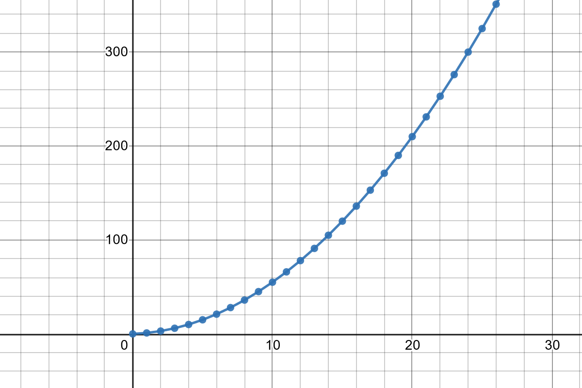
The triangle function looks a lot like a power function, though it’s a subtly distinct curve. It has a nice feature: \(f(x) - f(x-1) = x\). That is, the difference between one step and the next is the same as the value of the function at that next step.
This makes triangle numbers a very useful curve to apply to costs and milestones, like experience thresholds to level up or upgrading something with successive levels.
The triangle numbers are ingrained in Fallen London; to increase an attribute in FL, you need as many “change points” as the next level. So to go from, say, level 4 to 5, you need 5 change points; to get from 0 to 5, you will need \(T_5 = 15\) change points in total.
This intuitive property was also used in 3rd Edition Dungeons & Dragons, where the XP needed to get to a level \(x\) is \(1000 \times T_{x - 1}\). Therefore, the difference between your current level and the next is always 1000xp times your current level.
If a system exposes the numbers to players, this can be more graspable than a power function while still having many of the same properties.
The Sigmoid Curve
A “sigmoid” is any s-shaped curve. A sigmoid starts at some lower bound, rises steadily, and then smoothly plateaus at some upper bound.
There are many functions with a roughly sigmoid shape, but I’ll talk here about two: The logistic function, \(f_l\), and the algebraic sigmoid \(f_s\).
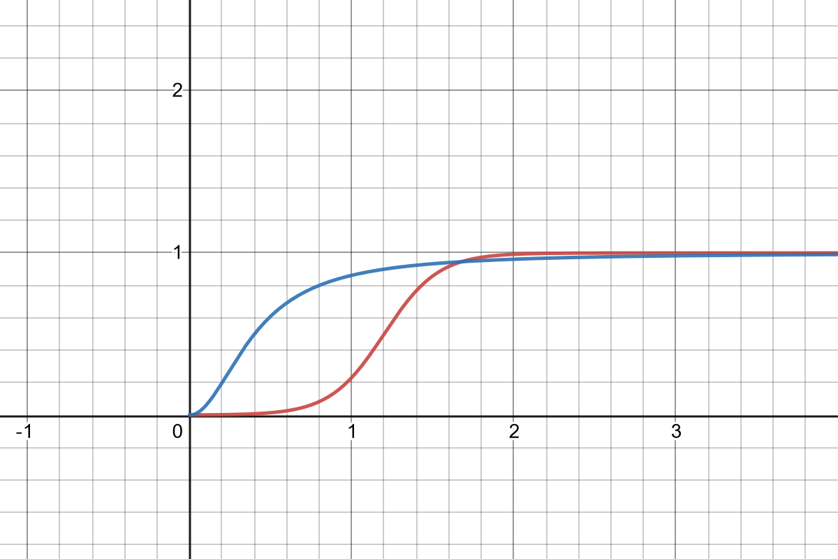
Above: \(f_l\), in red, and \(f_s\), in blue. Both functions have had their coefficients adjusted so they would mostly line up.
First, the algebraic sigmoid, which has a simpler expression:
\[f_s(x) = \frac{x^\lambda}{\sigma^\lambda + x^\lambda}\]
As far as I know, this sigmoid was first described in the context of game design by James Furness. It’s a normalized curve; it always ranges from \(0\) when \(x = 0\) on to \(1\) at some point when \(x\) is large enough.
The two coefficients, \(\sigma\) and \(\lambda\), respectively determine how big \(x\) has to be before the curve reaches its lower bound, and how steeply the curve rises to that point.
There are a lot of nice things about this curve, including that it’s inherently normalized. It also has a useful asymmetry, in that the it starts climbing quickly but plateaus relatively slowly.
The logistic function is widely used in statistical modeling. The traditional parametrized definition is:
\[ f_l(x) = \frac{L}{1 + e^{-k(x-x_0)}}\]
There are a lot of coefficients here, but the nice thing about the logistic function is that all of them have very well-defined effects.
- \(L\) is the upper bound, the number the function converges to for high values of \(x\).
- \(k\) is a coefficient that determines how steeply the curve rises; you can make this a negative number to invert the slope of the function and get a logistic decay curve.
- \(e\) is Euler’s number, of course, but for our purposes it’s just an arbitrary base. You could use any number greater than \(1\), though adjusting this value is completely equivalent to adjusting \(k\).
- \(x_0\) is a simple additive coefficient that shifts the curve left or right as desired. The inflection point of the curve is wherever \(x_0\) is set – that is, the midpoint in the rise is exactly at that point.
Besides the difference in how easy they are to compute, the main difference is in their skew. The algebraic sigmoid skews early, front-loading the effect of \(x\); the logistic function is perfectly symmetrical.
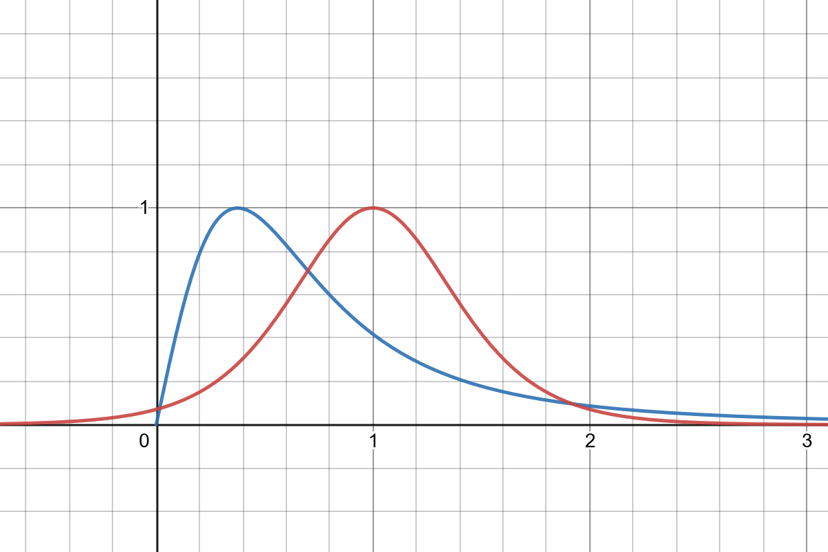
Above: A graph of the derivatives of the two sigmoid functions. They are both bell curves, but the algebraic sigmoid’s “bump” is noticeably skewed to the left.
What are sigmoids good for? Well:
- First, they are normalization functions; they will take an unbounded input and spit out a bounded output. Depending on the kinds of values you expect for the input, that output might not contain a lot of information about the original input, of course.
- Because of their bounded output, sigmoids are great for implementing caps and limits on the growth of something, or for smoothing between two values.
Some examples of this:
- Damage faloff: It’s very simple to define a logistic curve between, say, 0.5 and 1, which multiplies the damage done by a weapon based on the distance to the target. The logistic function is useful here because different weapons could have different ranges and more or less sharp faloff curves by adjusting \(k\) and \(x_0\).
- Speed bonus: On a game with scoring and leaderboards, a logistic curve could be used to scale a speed bonus based on a par time for the level. Players who complete the level very fast would get the maximum bonus; players who complete the level very slowly would get nothing. In this case, \(x\) is the completion time, and \(k\) is negative, inverting the curve’s slope.
- NPC disposition: Your game is a social simulation and it works by stacking NPC disposition modifiers on top of each other, like Crusader Kings 3. Using a sigmoid can be useful for normalizing an unbounded number into a bounded value, for example as an input to a facial animation system.
In conclusion…
Again, this is a bestiary; a limited selection of interesting specimens. There are more use cases and examples than the ones here, but I hope those work as a useful starting point for folks.
If you have a question, want to point out an error, or have a suggestion of something I didn’t include, the best place to ask questions is through tumblr.
I’m not the first to apply any of those ideas to game design, and a lot of this is widely known at least in some subset of the industry. Much of my thinking here (and desire to document it) has emerged from conversations with colleagues, in particular Emily Short, who originally pointed out the logistic curve to me.
This article is also inspired by some other pieces on the subject: